Getting started
PTArcade streamlines the implementation of Bayesian inference analyses for PTA data by providing an easy-to-use wrapper of ENTERPRISE and Ceffyl.
Already confused? Let's try to be more concrete. Say you have a new-physics model that produces a gravitational-wave background with a relic abundance given by \(\Omega_{\textrm{GW}}(f;\,\vec{\theta})\), where \(\vec{\theta}\) is a set of parameters describing the signal. You might now be interested in knowing if there are regions in the \(\vec{\theta}\) parameter space that could reproduce the signal observed in PTA data.1 PTArcade will allow you to answer this question in under 10 minutes (plus computational time) using real PTA data and the same statistical tools used by PTA collaborations.
The only thing that is asked of the user is to define the GWB produced by their model and the prior distribution of the model parameters. This is done via, what we call, a model file. Let's consider the specific example where
In this case, the model file will look something like this
from ptarcade.models_utils import prior

parameters = {# (1)!
            'log_A_star' : prior("Uniform", -14, -6), # (4)!
            'log_f_star' : prior("Uniform", -10, -6)
            }

def S(x):
    return 1 / (1/x + x)

def spectrum(f, log_A_star, log_f_star):  # (2)!
    A_star = 10**log_A_star
    f_star = 10**log_f_star

    return A_star * S(f/f_star) # (3)!
-
The parameter priors are defined via a dictionary named
parameters. The keys of this dictionary will be the names of the model parameters, and the values are parameter objects specifying the parameter prior distributions. -
The GWB spectrum is defined via the
spectrumfunction. The first argument of this function has to be calledfand is supposed to be an array of frequencies (in units of Hz) at which the spectrum will be evaluated. The remaining parameters should be named like the keys of theparametersdictionary. -
For any given set of new-physics parameters, in this example
log_A_starandlog_f_star, thespectrumfunction should return an array which contains the value of \(h^2\Omega_{\textrm{GW}}\) evaluated at those parameter values and at all the frequencies contained in theflist. -
Use any prior from [enterprise.signals.parameter][] or ptarcade.models_utils.
Once you have defined the model file, you can feed it to PTArcade by running it in a terminal
- The argument passed to the
-minput flag should be the path to the model file. Here, we are assuming that the model file is namedmodel_file.pyand is located in the folder from which we are running PTArcade.
This will implement and run the analysis, whose results are Markov chains that can be used to derive posterior distributions for the parameters of our model. For the example that we are considering, this yields the result:
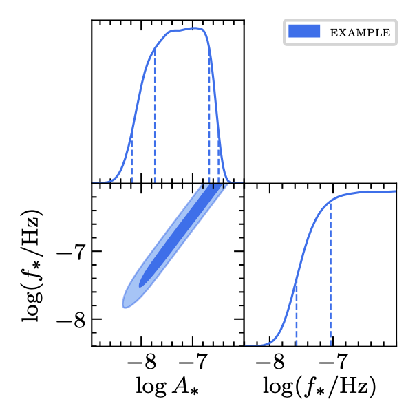
The lower left panel shows the 68% and 95% levels of the 2D posterior distribution for the \(\log_{10}A_*\) and \(\log_{10}(f/{\rm Hz})\) parameters. The other two panels report 1D marginalized posterior distributions. The dashed vertical lines in the plots for the 1D distributions indicate the 68% credible intervals.
Deterministic signals
PTArcade can also be used with deterministic signals. In this case, the user will have to specify the signal time series instead of the signal power-spectrum in the model file. See here for more details.
The chains produced by PTArcade can also be used to derive excluded regions of the parameter space and to perform model selection against the standard astrophysical interpretation of the PTA signal in terms of supermassive black-hole binaries.
After this high-level summary of what PTArcade can do, in the next sections, we will discuss:
- How to install PTArcade (locally, or on a cluster)
- How to define a model file
- How to change the parameters of PTArcade runs (PTA dataset, number of MC points, ...) using a configuration file
- The structure of the PTArcade outptut
- PTArcade utilities that can help in constructing model files or analyzing and plotting the MC chains.
How to cite PTArcade
If you use PTArcade in your work, please cite
@article{andrea mitridate_2023,
    title={PTArcade},
    DOI={10.5281/zenodo.7876430},
    publisher={Zenodo},
    author={Andrea Mitridate},
    year={2023},
    month={Apr},
    copyright = {Open Access}}

@article{Mitridate:2023oar,
    author = {Mitridate, Andrea and Wright, David and von Eckardstein, Richard and Schr\"oder, Tobias and Nay, Jonathan and Olum, Ken and Schmitz, Kai and Trickle, Tanner},
    title = "{PTArcade}",
    eprint = "2306.16377",
    archivePrefix = "arXiv",
    primaryClass = "hep-ph",
    month = "6",
    year = "2023"}
Additional Citations
PTArcade can be run in two modes: Ceffyl and ENTERPRISE (for more details on how to choose differnt run modes see here).
If you use PTArcade in Ceffyl mode (which is the default one), please also cite
@article{lamb2023rapid,
    title={Rapid refitting techniques for Bayesian spectral characterization of the gravitational wave background using pulsar timing arrays},
    author={Lamb, William G and Taylor, Stephen R and van Haasteren, Rutger},
    journal={Physical Review D},
    volume={108},
    number={10},
    pages={103019},
    year={2023},
    publisher={APS}
}
If you use PTArcade in ENTERPRISE mode, please also cite
@misc{enterprise,
    author       = {Justin A. Ellis and Michele Vallisneri and Stephen R. Taylor and Paul T. Baker},
    title        = {ENTERPRISE: Enhanced Numerical Toolbox Enabling a Robust PulsaR Inference SuitE},
    month        = sep,
    year         = 2020,
    howpublished = {Zenodo},
    doi          = {10.5281/zenodo.4059815},
    url          = {https://doi.org/10.5281/zenodo.4059815}
    }

@misc{enterprise-ext,
    author       = {Stephen R. Taylor and Paul T. Baker and Jeffrey S. Hazboun and Joseph Simon and Sarah J. Vigeland},
    title        = {enterprise_extensions},
    year         = {2021},
    url          = {https://github.com/nanograv/enterprise_extensions},
    note         = {v2.3.3}
    }